MagSense — Multi-Sensor Magnetic-Field Imaging Platform
An experimental instrumentation platform designed to evaluate multi-point spatial magnetic-field acquisition, real-time bicubic gradient heatmap rendering, and the transition from loose breakout wiring to an autonomous 6-layer edge-computing instrument.
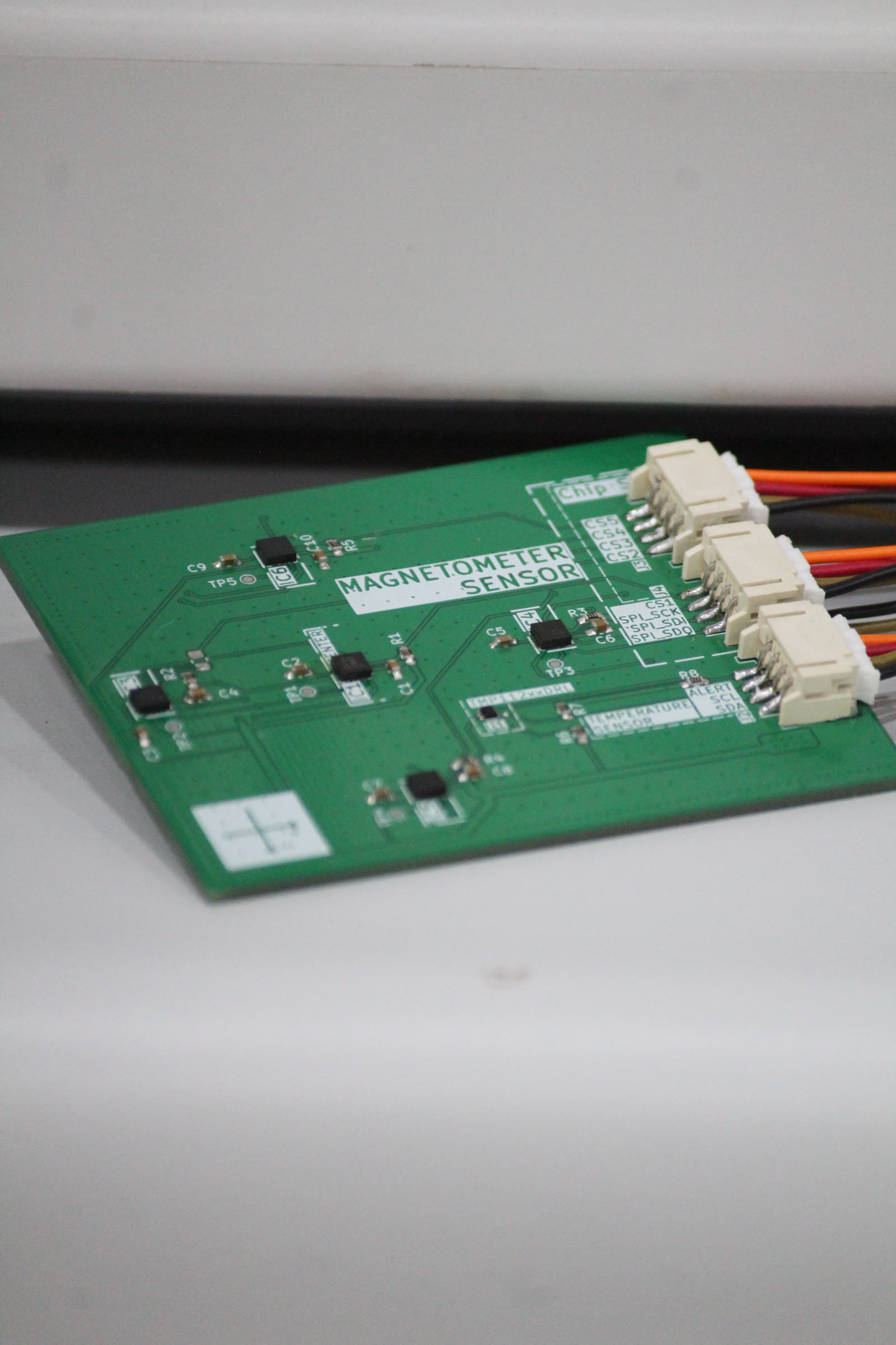
ENGINEERING MOTIVATION & FULL SPECIFICATIONS expand_more
Engineering Motivation: Traditional magnetometers capture only single-point flux density vectors B⃗ = (Bx, By, Bz), making it impossible to separate background geomagnetic bias from local dipole position, field curvature, or gradient anomalies.
MagSense addresses this by distributing five anisotropic magnetoresistive (AMR) sensors in a cross formation (r = 20 mm). In Revision 1, an external ESP32 controller streams high-speed binary packets to a custom Python/PySide6 visualizer. In Revision 2 (Megnito), the architecture is redesigned into a monolithic 6-layer PCB with an onboard STM32G431 MCU, CAN-FD, native USB-C, and intelligent power multiplexing.
Engineering Motivation: Traditional magnetometers capture only single-point flux density vectors B⃗ = (Bx, By, Bz), making it impossible to separate background geomagnetic bias from local dipole position, field curvature, or gradient anomalies.
MagSense addresses this by distributing five anisotropic magnetoresistive (AMR) sensors in a cross formation (r = 20 mm). In Revision 1, an external ESP32 controller streams high-speed binary packets to a custom Python/PySide6 visualizer. In Revision 2 (Megnito), the architecture is redesigned into a monolithic 6-layer PCB with an onboard STM32G431 MCU, CAN-FD, native USB-C, and intelligent power multiplexing.
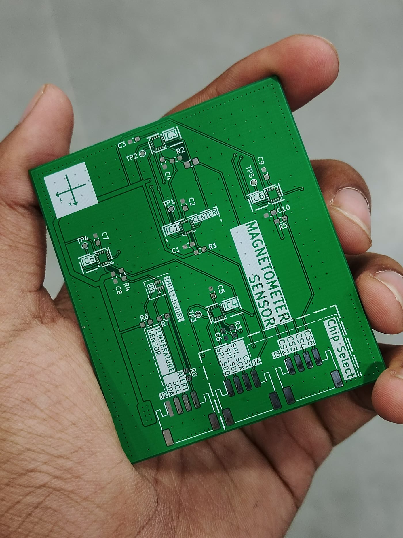
Measurement Concept & Five-Sensor Cross Geometry
Standard 3-axis magnetometers cannot differentiate between a homogeneous ambient magnetic field (such as Earth's geomagnetic flux) and a localized magnetic field disturbance caused by a nearby ferromagnetic object or permanent magnet. MagSense solves this by implementing a five-point differential spatial array.
The 20 mm Equilateral Cross Layout
The array places one MMC5983MA sensor at the coordinate origin (0, 0) as a central reference baseline, with four peripheral sensors placed along orthogonal axes at a radial distance of r = 20.00 mm:
Spatial Gradient & Anomaly Detection Formulations
By taking differential readings between opposite sensor pairs separated by Δd = 40.00 mm, common-mode ambient fields cancel out, isolating the local field gradient tensor components:
When a magnetic anomaly moves over the array, these second-order differences generate localized peaks and troughs, providing the mathematical input data required to project continuous flux heatmaps.
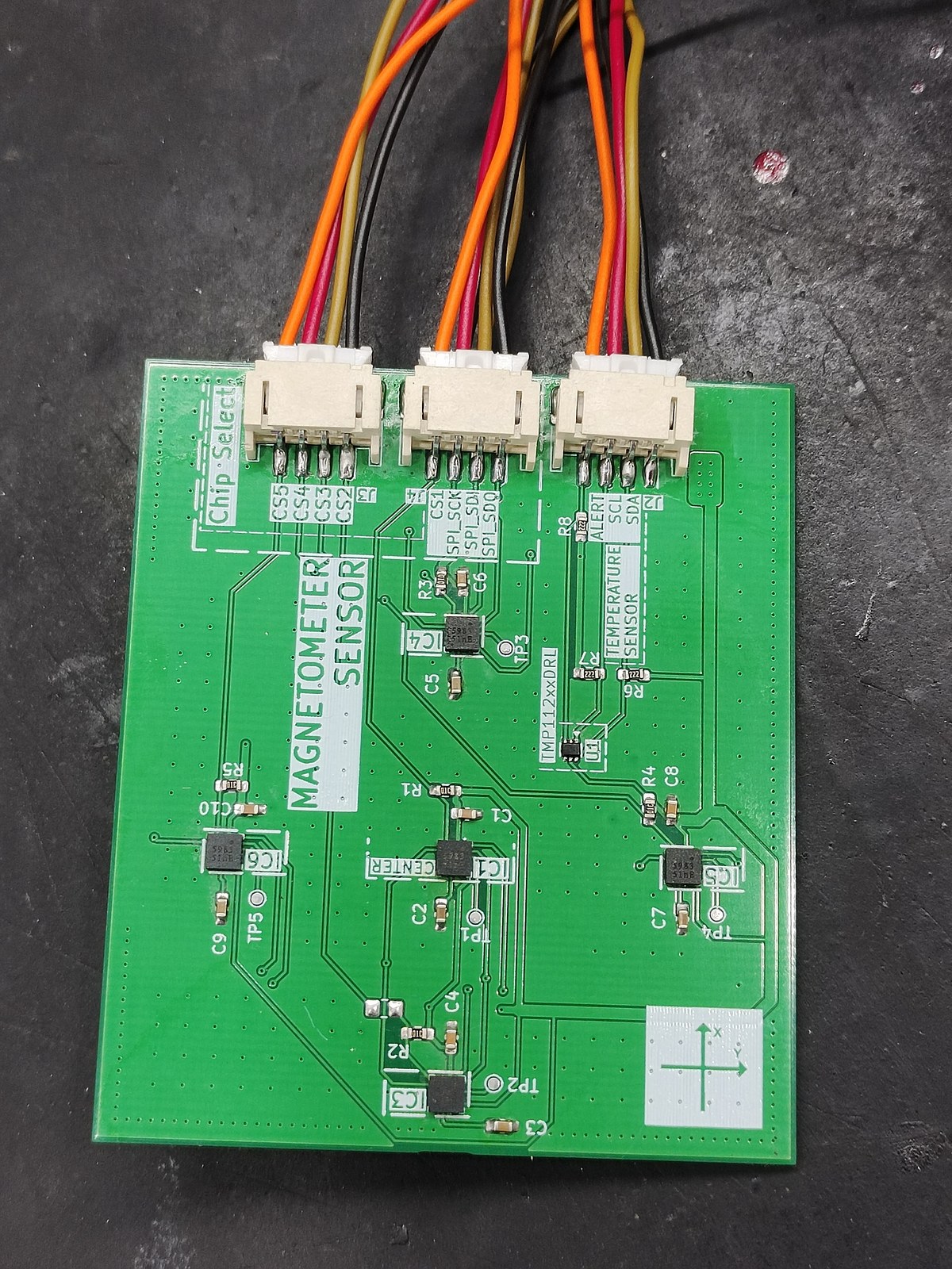
Revision 1 Hardware & Embedded Acquisition Architecture
Revision 1 was realized as a modular two-board system: a dedicated sensor carrier PCB connected to an external ESP32 DevKit V1 controller via a 15-conductor JST-XH wiring loom.
Hardware Pinout & Bus Topology
All five MMC5983MA sensors share common clock, data-in, and data-out SPI lines, while five dedicated GPIO pins provide individual active-LOW chip select control. The TMP112 sensor communicates over a separate two-wire I²C bus.
| Signal | ESP32 Pin | Target Destination | Mode / Spec |
|---|---|---|---|
| SCK | GPIO 18 | All 5 MMC5983MA ICs | Shared Bus (100 kHz) |
| MISO | GPIO 19 | All 5 MMC5983MA ICs | Shared Data Return |
| MOSI | GPIO 23 | All 5 MMC5983MA ICs | Shared Command Line |
| CS_Center | GPIO 5 | Center Sensor (IC1) | Active LOW |
| CS_Bottom | GPIO 32 | Bottom Sensor (IC5) | Active LOW |
| CS_Top | GPIO 27 | Top Sensor (IC6) | Active LOW |
| CS_Right | GPIO 13 | Right Sensor (IC4) | Active LOW |
| CS_Left | GPIO 25 | Left Sensor (IC3) | Active LOW |
| I2C_SDA | GPIO 21 | TMP112 Sensor | Addr 0x48 (400 kHz) |
| I2C_SCL | GPIO 22 | TMP112 Sensor | Addr 0x48 (400 kHz) |
Empirical Engineering Reality: Harness Parasitics
During bench bring-up, the unshielded 15-wire jumper harness introduced significant parasitic capacitance and ground-bounce inductance. Attempting to clock the SPI bus at 4 MHz or 10 MHz caused bit slippage and MISO corruption.
Practical Solution: The SPI bus was conservatively throttled to 100 kHz Mode 0 in firmware (main.cpp). Because 5 sensors × 6 bytes of measurement data require only 30 bytes per frame, 100 kHz provided more than enough bandwidth to achieve 102.1 Hz sampling while guaranteeing 100% signal integrity.
Binary Pipeline & FreeRTOS Task Architecture
Firmware is written in modern C++ with PlatformIO. Acquisition is managed by a high-priority FreeRTOS task pinned to ESP32 Core 1 (StreamingTask.cpp) to avoid contention with USB serial interrupts:
#pragma pack(push, 1)
struct SensorPacket {
uint32_t timestampUs; // 4 bytes: Boot timestamp
float temperatureC; // 4 bytes: TMP112 °C
float magX[5]; // 20 bytes: Center, B, T, R, L
float magY[5]; // 20 bytes: Center, B, T, R, L
float magZ[5]; // 20 bytes: Center, B, T, R, L
uint8_t activeSensorsBitmask; // 1 byte: Health mask (bits 0-4)
};
#pragma pack(pop)
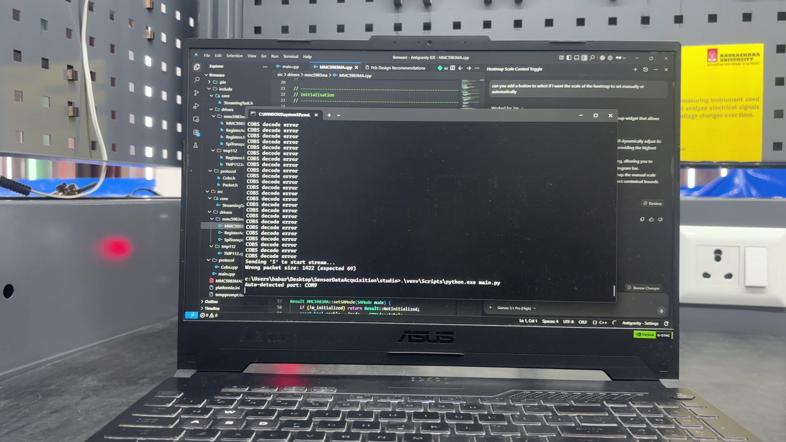
MagSense Studio — Live Visualization & Video Evidence
The PC client is built using Python, PySide6 (Qt6), PyQtGraph, PyOpenGL, NumPy, and SciPy. Below is the authentic bench testing recording demonstrating live dynamic field projection.
Heatmap Math: Sparse Grid to Spline Surface
It is vital to understand how the visualizer turns five discrete point sensors into a smooth 2D heatmap. In heatmap_2d.py:
- 1. Scalar Vector Calculation: Each sensor computes total flux magnitude |B| = √(Bx2 + By2 + Bz2) or inclination dip angle.
-
2. 3×3 Grid Mapping: The five values are assigned to grid cells:
Center=(1,1), Top=(0,1), Bottom=(2,1), Left=(1,0), Right=(1,2)
-
3. Synthetic Corner Averaging: The four missing corners are calculated by averaging adjacent orthogonal sensors:
Grid[0,0] = (Top + Left) / 2.0
-
4. High-Resolution Spline Zoom: The 3 × 3 grid is upscaled by a factor of 80 using third-order bicubic spline interpolation:
scipy.ndimage.zoom(grid, 80, order=3)
Revision 2 — The Megnito Monolithic Instrument
While Revision 1 successfully validated the 5-sensor acquisition pipeline, loose jumper wiring and an external DevKit limited robustness and industrial integration. The second iteration—named Megnito—integrates the entire instrument into an autonomous 6-layer high-density PCB.
STM32G431CBTx MCU
Arm Cortex-M4F core clocked at 170 MHz with hardware floating-point unit (FPU) and DSP acceleration. Replaces the external ESP32, enabling local finite-difference gradient calculations and DMA-driven continuous SPI streaming.
6-Layer Shielded Stackup
Compact 50.05 × 50.05 mm square footprint with M2 mounting holes. Symmetrical 6-layer stackup featuring solid internal ground planes (In1.Cu and In4.Cu) to shield sensitive AMR sensors from high-speed digital switching transients.
Auto-Switching Power Mux
TI TPS2115ADRBT power multiplexer (IC7) autonomously switches between USB-C 5V and external battery power (J4, JST-PH 2.0 mm LiPo header) without resetting the MCU. Backed by a TI TPS7A0233DBVR ultra-low-noise 3.3V LDO (IQ = 25 nA).
CAN-FD & Daisy Chaining
Infineon TLT9251VLEXUMA1 automotive-grade CAN transceiver (IC8) enables robust differential communication over long distances. Features an onboard switchable 120 Ω termination resistor (R13, 2512 package) via solder jumper JP1.
USB-C & Qwiic Ecosystem
16-pin USB Type-C receptacle (J5) protected by a ST USBLC6-2SC6 low-capacitance ESD clamp array (U3). Includes a SparkFun Qwiic I²C connector (J1), auxiliary SPI2 header (J2, 5-pin), and dedicated 3-pin UART debug port (J6).
RGB Telemetry & Tare Button
A WS2812B-2020 miniature addressable RGB LED (D4) is placed at (84.52, 89.15) mm immediately adjacent to the central sensor for dynamic optical alerts. A low-profile C&K PTS815 tactile switch (S1) provides physical zeroing/tare control.
| Layer | Type | Thickness | Material | Primary Engineering Function |
|---|---|---|---|---|
| F.Cu (L1) | Copper (Outer) | 35 µm (1 oz) | Copper | Component pads, decoupling caps, local high-speed routing |
| Dielectric 1 | Prepreg | 100 µm | FR4 (εr = 4.5) | High-frequency isolation between signals and ground |
| In1.Cu (L2) | Copper (Inner) | 35 µm (1 oz) | Copper | Solid Ground Reference Plane (GND) — Low return inductance |
| Dielectric 2 | Core | 535 µm | FR4 (εr = 4.5) | Rigid structural substrate core |
| In2.Cu (L3) | Copper (Inner) | 35 µm (1 oz) | Copper | Internal high-speed SPI bus & CAN differential pairs |
| Dielectric 3 | Prepreg | 100 µm | FR4 (εr = 4.5) | Center layer dielectric spacer |
| In3.Cu (L4) | Copper (Inner) | 35 µm (1 oz) | Copper | Power distribution rails (+3.3V, 5V, VIN) & control lines |
| Dielectric 4 | Core | 535 µm | FR4 (εr = 4.5) | Rigid structural substrate core |
| In4.Cu (L5) | Copper (Inner) | 35 µm (1 oz) | Copper | Solid Ground Shield Plane (GND) — Magnetic isolation |
| Dielectric 5 | Prepreg | 100 µm | FR4 (εr = 4.5) | Bottom prepreg bonding layer |
| B.Cu (L6) | Copper (Outer) | 35 µm (1 oz) | Copper | Bottom ground shield pour, connector escapes, test points |
Empirical Validation, Calibration Status & Boundaries
In keeping with strict engineering rigor, this section explicitly delineates what has been experimentally proven on physical hardware versus what remains an unvalidated design specification.
| Claim / Subsystem | Current Verification Status | Primary Evidence in Workspace | Remaining Boundaries / Unproven Aspects |
|---|---|---|---|
| Rev 1 Multi-Sensor SPI | Verified in Hardware | magsense-live-test.mp4, main.cpp | Throttled to 100 kHz due to harness line parasitics. |
| COBS Serial Pipeline | Verified in Software | magsense-studio-heatmap.jpg | Requires initial 'S' handshake to start streaming. |
| Dynamic Anomaly Tracking | Verified in Video | magsense-live-test.mp4 (6.37s) | Qualitative response only; field intensity is uncalibrated. |
| Bicubic Heatmap Rendering | Verified in Python | heatmap_2d.py, requirements.txt | Corners are mathematically synthesized; not physical nodes. |
| Absolute Field Calibration | Uncalibrated / Missing | No calibration logs or chamber data | Uses datasheet nominal sensitivity only (16384 counts/G). |
| Thermal Compensation | Partial (Telemetry Only) | TMP112 read in Packet.h | Temperature is transmitted but not applied to drift equations. |
| Rev 2 Megnito Board | CAD & Gerbers Complete | Megnito.kicad_pcb, Megnito-job.gbrjob | Unfabricated. Zero physical board testing or bring-up logs. |
The MagSense platform currently functions as a spatial field anomaly and gradient visualizer, not a certified laboratory magnetometer. No 3-axis Helmholtz coil tests, zero-gauss mu-metal chamber baseline calibrations, or hard/soft-iron ellipsoid corrections have been performed on the physical assembly. All numeric Tesla/Gauss values are derived strictly from MEMSIC nominal factory conversion parameters.
Lessons Learned & Development Roadmap
Developing the MagSense prototype provided valuable practical lessons in high-speed sensor buses, sparse matrix interpolation, and the engineering trade-offs of modular breakouts versus monolithic integration.
Harness Capacitance Dominates
Jumper wires and unshielded ribbon cables introduce severe parasitics that ruin SPI rise times across multi-drop nodes. While throttling clock frequency is a valid bench workaround, physical board integration with controlled ground planes is the only true engineering solution.
Bicubic Interpolation Traps
Third-order spline interpolation produces visually striking heatmaps that can easily mislead observers into believing high spatial sensor density exists. Engineers must maintain clear distinction between real spatial measurements and mathematical surface approximations.
Protocol Decoupling Pays Off
Adopting a packed C++ binary struct with COBS framing over high-speed UART (921,600 baud) kept MCU loop execution deterministic and lightweight, leaving computation-heavy matrix math and OpenGL rendering to the desktop client.